Quadrotor Control

Summary

Quadrotor dynamics, when simplified to exclude drag effects, center of mass deviations, and other disturbances, can be modeled by the following differental equations: \[ \begin{align} m \ddot{\mathbf{r}} &= -mg \vec{e}_3 + f_c ^\mathcal{W}\!\boldsymbol{R}_\mathcal{B} \vec{e}_3, \\ \mathcal{I} \dot{\boldsymbol{\omega}} &= -\boldsymbol{\omega} \times \mathcal{I} \boldsymbol{\omega} + \boldsymbol{\tau}, \end{align} \] where \(\mathbf{r}\) is the robot's position, \(\boldsymbol{\tau}\) is the torque, \(\boldsymbol{\omega}\) is its angular velocity, \(^\mathcal{W}\!\boldsymbol{R}_\mathcal{B}\) is the rotation from the world frame \(\mathcal{W}\) to the body frame \(\mathcal{B}\), and \(\vec{e}_3 = [0, 0, 1]^\top\). For any linear controller, we can linearize these equations about a hover condition as in [1], giving us linear approximations of the quadrotor's dynamics, defined by: \[ \begin{align} \ddot{z}_W \approx \frac{1}{m}(f_c-mg), \quad &\ddot{x}_B \approx \theta g, \quad \ddot{y}_B \approx - \phi g, \\ \ddot{\phi} \approx \frac{\tau_x}{I_x}, \quad \ddot{\theta} &\approx \frac{\tau_y}{I_y}, \quad \ddot{\psi} \approx \frac{\tau_z}{I_z}. \end{align} \] We can then formulate a state-space model with the inner and outer loop states defined as \[ \begin{align*} \mathbf{x}_\text{outer} &= \begin{bmatrix} \mathbf{r} & \mathbf{\dot{r}} \end{bmatrix}^\top, \\ \mathbf{x}_\text{inner} &= \begin{bmatrix} \boldsymbol{\eta}_{_\text{ZYX}} & \boldsymbol{\dot{\eta}}_{_\text{ZYX}}\end{bmatrix}^\top, \end{align*} \] with control vectors: \[ \begin{align*} \mathbf{u}_\text{outer} &= \begin{bmatrix} f_c & \theta_\text{des} & \phi_\text{des} \end{bmatrix}^\top, \\ \mathbf{u}_\text{inner} &= \begin{bmatrix} \tau_x & \tau_y & \tau_z \end{bmatrix}^\top. \end{align*} \] Formulating the system this way, we can form the state-space equations: \[ \begin{align*} \mathbf{\dot{x}}_\text{outer} &= \mathbf{A}_o \mathbf{x}_\text{outer} + \mathbf{B}_o \mathbf{u}_\text{outer}, \\ \mathbf{\dot{x}}_\text{inner} &= \mathbf{A}_i \mathbf{x}_\text{inner} + \mathbf{B}_i \mathbf{u}_\text{inner}. \end{align*} \] To control this linearized system with an Linear Quadratic Regulator (LQR), we define the control law: \[ \mathbf{u}(t) = -\mathbf{Kx}(t) \] where \(\mathbf{K}\) ensures the minimization of the objective function \[ J = \int_0^\infty \left( \mathbf{x}^\top \mathbf{Qx} + \mathbf{u}^\top \mathbf{Ru} \right) dt \] where \(\mathbf{Q}\) is the state weighting matrix and \(\mathbf{R}\) is the control weighting matrix. Luckily, there is a closed-form solution to this minimization problem, namely \[ \mathbf{K} = \mathbf{R}^{-1} \mathbf{B}^\top \mathbf{P} \] where \(\mathbf{P}\) is the solution to the Algebraic-Riccati equation \[ \mathbf{A}^\top \mathbf{P} + \mathbf{PA} - \mathbf{PBR}^{-1}\mathbf{B}^\top\mathbf{P} + \mathbf{Q} = 0. \] It is important we choose reasonable state and control weighting matrices because they define (along with the linearized dynamic constraints), the solution to this optimization problem. After some tuning, the optimal \(\mathbf{K}\) can be found for both loops.

Testing

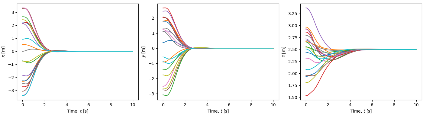
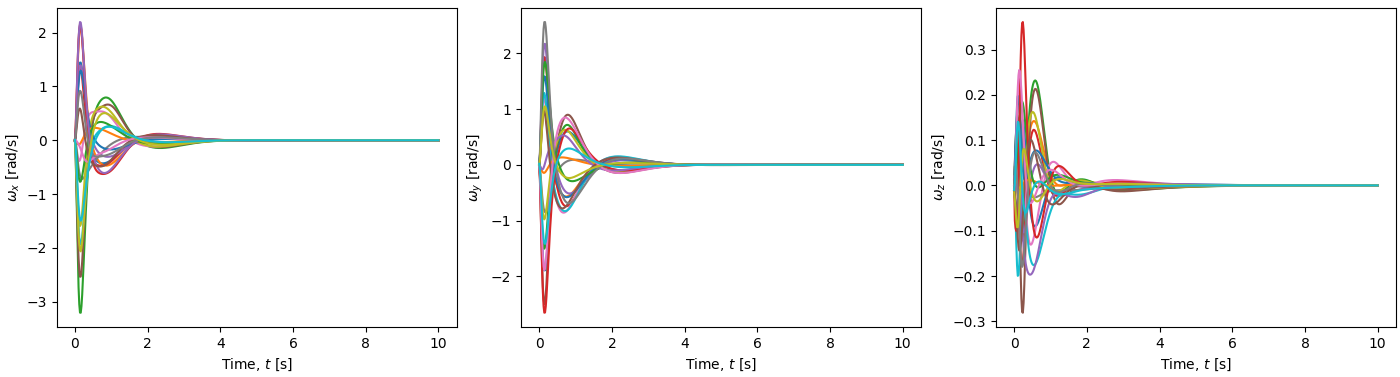
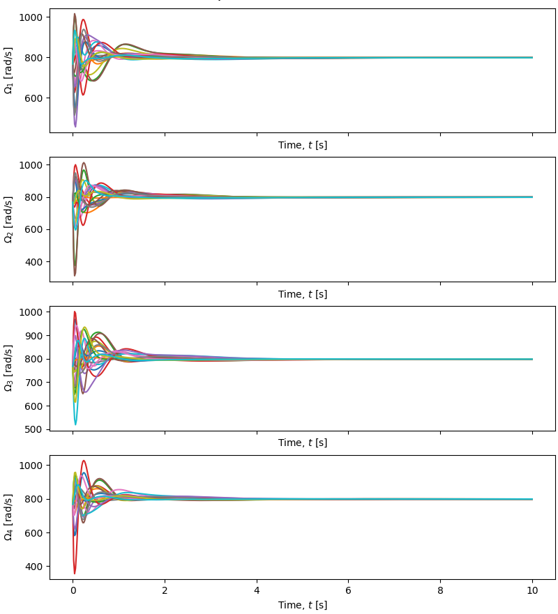
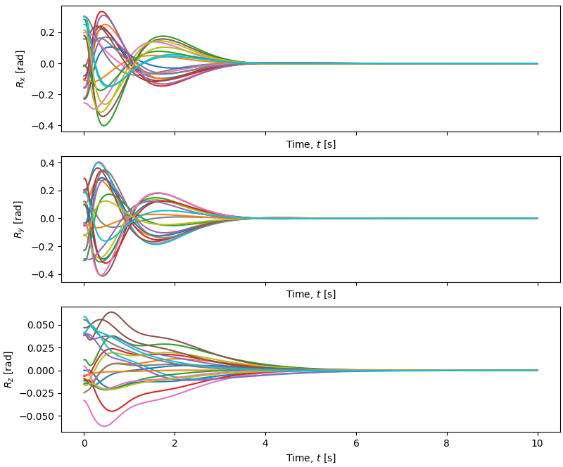
We can test the performance of the controller on various quadrotors initialized at states within a reasonable range for the small-angle approximation to hold. Such tests produce the following results in a lightweight simulator.

Quadrotor Position Response

Quadrotor Body Rate Response

Quadrotor Motor Rates

Quadrotor Angular Response

Citations

[1] L. Martins, C. Cardeira, and P. Oliveira, “Linear quadratic regulator for trajectory tracking of a quadrotor,” IFAC-PapersOnLine, vol. 52, no. 12, pp. 176–181, 2019, 21st IFAC Symposium on Automatic Control in Aerospace ACA 2019. [Online]. Available: https://www.sciencedirect.com/science/article/pii/S2405896319311450